Linear Feedback Shift Registers for the Uninitiated, Part XI: Pseudorandom Number Generation
Last time we looked at the use of LFSRs in counters and position encoders.
This time we’re going to look at pseudorandom number generation, and why you may — or may not — want to use LFSRs for this purpose.
But first — an aside:
Science Fair 1983
When I was in fourth grade, my father bought a Timex/Sinclair 1000. This was one of several personal computers introduced in 1982, along with the Commodore 64. The T/S-1000 was this ugly little flat computer with an ugly little flat keyboard and 2 kilobytes of RAM:
For a display, you had to connect it to a television’s antenna jack through a VHF switch, so that you didn’t have to unscrew the antenna leads every time you wanted to use the computer or go back to watching TV. (No HDMI cables back then.) The ugly little flat keyboard didn’t just look ugly, it felt ugly: the T/S-1000 used a so-called membrane keyboard. There was no key travel; it felt like pushing on a vinyl-covered wall. You pushed on the keys and maybe it registered a keypress. All it could do was run BASIC programs you typed in, and the only way to store these for later retrieval was to connect it to a cassette tape recorder’s microphone jack, stick in a blank cassette tape, type SAVE and press record on the cassette player, taking care to write down the number on the tape recorder’s counter so you could rewind it and LOAD the program back into the T/S-1000. Sometimes this worked. I seem to remember we got it from Kmart, probably in late December 1982 as part of a post-holiday clearance sale. A later purchase was a 16-kilobyte memory cartridge that sold for \$49.
If it sounds like I’m not speaking about our computer in glowing praise, well, that’s just the modern me showing my contempt for the thing. As a nine-year-old, the presence of a computer at home was a wonderful opportunity. I had first encountered a personal computer at school a year earlier; my third-grade teacher had me figure out how to use our school’s Tandy TRS-80 (the “Trash-80”), which got wheeled around on an audiovisual cart whenever one of the teachers wanted to borrow it. But to have a computer at home was another matter. I learned how to program in BASIC, which at the time was an end to itself; there really wasn’t much you could do that was useful on a T/S-1000. My dad taught me what sines and cosines were — or at least, enough about them to draw a circle in low-resolution graphics.
The August 1982 issue of Popular Science had this to say about the T/S-1000:
Timex’s closest competition is from Commodore. It’s scheduled to release its \$180 color-graphics and music-synthesizing Max computer by the time you read this. Says Mike Tomczyk, international product manager for the company, “I don’t see the Timex computer as much of a threat. If you want the cheapest thing, you have it. But there are so many things to consider. If it gets people into computing, it will help Commodore because they’ll want to move up. I see that as a benefit.”
Mr. Tomczyk was exactly right; we bought a Commodore 64 in the summer of 1983 and I never touched the T/S 1000 after that. (I’d never heard of the Commodore MAX. Looks like it never took off.)
Lest I have any nostalgia about our T/S 1000, I can always cure it by looking at the user manual, written by Mr. Steven Vickers, courtesy of Lewin Edwards’s collection of information about vintage computing. Here’s what the user manual has to say by way of an introduction:
Welcome to the world of computing. Before you plug in your new Timex/Sinclair 1000, please take a moment to think about this exciting new adventure. We want to assure you that:
You will enjoy computing.
You will find it easy as well as enjoyable.
You shouldn’t be afraid of the computer. You are smarter than it is. So is your parakeet, for that matter.
You will make mistakes as you learn. The computer will not laugh at you.
Your mistakes will not do any harm to the computer. You can’t break it by pushing the “wrong” button.
You are about to take a giant step into the future. Everyone will soon be using computers in every part of their daily lives, and you will have a head start.
You do not need to know how to program a computer to use the T/S 1000, any more than you need to know how to do a tuneup to drive a car. You may want to learn to program — it is not difficult and can be very enjoyable — but you can use the computer for the rest of your life without having to learn programming.
A computer is a tool, like a hammer or saw — or perhaps like a food processor. Hammers and saws generally do only one thing well. A food processor can perform different operations, and normally you can “program” it by simpling pushing the proper buttons. A computer is an information tool, and is the most versatile tool ever invented. Because it can do many things, it needs a sequence of instructions to perform any particular task. These instructions are called programs.
There are many available programs for your everyday use with your Timex/Sinclair 1000. You can use them for learning, and for home or business management (like balance-sheet calculations, record-keeping, accounting/bookkeeping, taxes, personal or business inventories, etc.) You can maintain athletic statistics, recipes, address or Christmas-card lists, prepare reports, learn and use mathematics, play games, and do many other things.
One of the most important uses of the Timex/Sinclair computer is as an educational tool. Right now your children are beginning to use computers in school. They are learning about computers, and they are using computers to help them learn other subjects. Your T/S 1000 can help your children learn at home, whether their schools have computers or not. Many educational programs are available, for both tutorial help and advanced learning. You can find all of these programs at the same store where you bought your Timex/Sinclair 1000. Many more programs are being developed right now for the T/S 1000, because it is the world’s best-selling computer. In the near future, your personal computer will be able to dial and answer your telephone, monitor your burglar alarm, control appliances, water your lawn and perform many other duties for you. Keep in touch with your dealer!
This is a bit of hyperbole by 1982 standards, but from today’s perspective Mr. Vickers was fairly accurate, and the attitude encouraged in the user manual (“You will enjoy computing. You will find it easy as well as enjoyable. You shouldn’t be afraid of the computer. You are smarter than it is....”) is something invaluable that everyone who aspires to be a programmer should keep in mind.
At any rate, I used our Timex/Sinclair in a science fair project a few months after we got it. I wrote a program to simulate a bunch of dice rolls, probably something like this:
10 DIM D(12)
20 FOR I=2 TO 12
30 LET D(I) = 0
40 NEXT I
50 FOR I=1 TO 1000
60 LET A = INT(RND*6) + 1
70 LET B = INT(RND*6) + 1
80 LET C = A+B
90 LET D(C) = D(C) + 1
100 NEXT I
110 FOR I=2 TO 12
120 PRINT I, D(I)
130 NEXT I
My attempt above to recreate the dice program is probably the first BASIC program with line numbers I’ve written in the last 27 years, and it leaves a bad taste in my mouth. I don’t really want to run it. (I had to qualify that statement “with line numbers” because from time to time I am forced to use Visual Basic with Microsoft products.) So here’s the same sort of thing in Python, along with an expected count:
import random

dice_history = [0]*13
Nrolls = 36000
for i in xrange(Nrolls):
    roll = random.randint(1,6) + random.randint(1,6)
    dice_history[roll] += 1
for i in xrange(2,13):
    expected_count = Nrolls * (6 - abs(i-7)) / 36
    print("roll %2d: %5d times (expected: %d)"
          % (i, dice_history[i], expected_count))
roll 2: 993 times (expected: 1000) roll 3: 2025 times (expected: 2000) roll 4: 2968 times (expected: 3000) roll 5: 4021 times (expected: 4000) roll 6: 5024 times (expected: 5000) roll 7: 6015 times (expected: 6000) roll 8: 5017 times (expected: 5000) roll 9: 3969 times (expected: 4000) roll 10: 2937 times (expected: 3000) roll 11: 2015 times (expected: 2000) roll 12: 1016 times (expected: 1000)
If you have studied probability, this is perhaps familiar to you: the number 7 is the most common roll of a pair of dice, because there are 6 ways to form it: 1+6, 2+5, 3+4, 4+3, 5+2, and 6+1. Whereas 2 and 12 are the least common rolls, requiring 1+1 and 6+6, respectively. So the probability of a 2 or 12 is 1/36, 3 or 11 is 2/36, 4 or 10 is 3/36, 5 or 9 is 4/36, 6 or 8 is 5/36, and 7 is 6/36.
I didn’t win any prize in that science fair, but I learned how to use the random number generator RND in BASIC, as well as some basic aspects of probability.
Random Number Generators: A Quick Primer
The first thing you should know about random number generators is that there’s no such thing as a random number. A number itself is not random; it can be chosen at random, by sampling from a particular distribution, and even then, as long as you use a deterministic algorithm, the samples are, at best, pseudorandom, meaning that they are an attempt to masquerade as random samples. The RND function in BASIC and the random.randint() function in Python are examples of functions called pseudorandom number generators (PRNGs) that are designed to mimic samples of a particular random distribution. RND and random.random() both are designed to produce values uniformly distributed between 0 and 1, including 0 but excluding 1. Mathematical notation for this is \( v \in [0,1) \) where \( v \) is a random variable and \( [0,1) \) represents a half-open interval, including the 0 and excluding the 1.
How well they mimic samples from this particular random distribution depends on a couple of things:
- what kind of “randomness” is required
- statistical randomness
- cryptographic randomness
- how the PRNG is implemented
- what algorithm is used
- where the seed came from
Statistical randomness means that if you take a whole bunch of sample outputs from the PRNG and compute summary statistics, these summary statistics are indistinguishable from the same statistics computed from truly random samples of the same distribution. Summary statistics are calculations that measure something about the sample set, like the mean or median or standard deviation or correlation between successive samples, so statistical tests of randomness compare the results to the expected values of these statistics given that distribution. For example, with dice rolls, the mean value should be close to 3.5, and the correlation between successive pairs of dice rolls should be close to zero. The theory of statistics allows you to compute some kind of probability that the random samples from the PRNG are indistinguishable from an actual set of random dice rolls.
Cryptographic randomness means that looking at past samples of the PRNG gives you no information about future samples, even if you know how the algorithm works. The distinction between statistical and cryptographic randomness is subtle, and to understand it, we need to know a little bit more about how PRNGs work.
All PRNGs are state machines: they contain some sort of state variable, and for each new sample, the state variable is updated and the output is a function of the PRNG state. The curious thing about a PRNG state machine — as opposed to state machines in general — is that there are no inputs*, just updates in state and output. The initial value of the PRNG state is called the seed, and in order to make sure the PRNG state is not predictable, the seed must come from some source of truly random data. In a PRNG, the outputs are deterministic functions of the seed, so using the same seed twice will produce the same sequence of outputs.
(*Some algorithms like Yarrow do periodically draw from external sources to “reseed” and maintain unpredictability.)
One example of a PRNG is a linear congruential generator or LCG, where we update the PRNG state as follows:
$$S_n = (aS_{n-1} + c) \bmod m$$
for some fixed values of \( a, c, \) and \( m \). For example, if I used \( a = 2718, c = 3141, m = 2^{16} \) and an initial seed \( S_0 = 0 \), then the values of \( S_n \) evolve as follows:
a = 2718
c = 3141
m = 1 << 16
S = 0
for k in xrange(20):
    print "S[%2d] = %5d" % (k, S)
    S = (a*S+c) % m
S[ 0] = 0 S[ 1] = 3141 S[ 2] = 20699 S[ 3] = 33135 S[ 4] = 17607 S[ 5] = 17687 S[ 6] = 38519 S[ 7] = 36791 S[ 8] = 58679 S[ 9] = 43575 S[10] = 16439 S[11] = 54327 S[12] = 11319 S[13] = 31799 S[14] = 56375 S[15] = 7223 S[16] = 39991 S[17] = 39991 S[18] = 39991 S[19] = 39991
And, of course, that fails, because the state got stuck in a repeating cycle. We could swap \( a \) and \( c \):
a = 3141
c = 2718
m = 1 << 16
S = 0
for k in xrange(50):
    print "S[%2d] = %5d" % (k, S)
    S = (a*S+c) % m
S[ 0] = 0 S[ 1] = 2718 S[ 2] = 20276 S[ 3] = 54178 S[ 4] = 44360 S[ 5] = 7942 S[ 6] = 44860 S[ 7] = 5578 S[ 8] = 25104 S[ 9] = 14574 S[10] = 35524 S[11] = 41330 S[12] = 58968 S[13] = 16470 S[14] = 27084 S[15] = 7834 S[16] = 33312 S[17] = 40254 S[18] = 21588 S[19] = 46402 S[20] = 64872 S[21] = 14246 S[22] = 53852 S[23] = 3434 S[24] = 41008 S[25] = 30606 S[26] = 60388 S[27] = 20242 S[28] = 12920 S[29] = 17654 S[30] = 10476 S[31] = 8762 S[32] = 64576 S[33] = 2014 S[34] = 37236 S[35] = 44770 S[36] = 50568 S[37] = 43078 S[38] = 44412 S[39] = 40202 S[40] = 54864 S[41] = 36398 S[42] = 34052 S[43] = 5298 S[44] = 63128 S[45] = 41366 S[46] = 40972 S[47] = 48602 S[48] = 28256 S[49] = 19070
and this looks better, but notice that the state values are always even numbers; the least significant bit is never 1, and that’s a drawback because we essentially waste one of the state bits. Because all PRNGs have finitely many bits of state, they must eventually produce a cycle (same state = same output sequence), and the period of a PRNG is ideally \( 2^N \) where there are \( N \) bits of state. To do this requires some careful design, and even then, many PRNGs have been found to have flaws. Today’s garden-variety PRNG, used in many applications including Python’s random module, is the Mersenne Twister, with period \( 2^{19937}−1 \); with properly generated seed, this won’t repeat anytime during the lifetime of the universe, and it has reasonably good statistical properties.
The Timex/Sinclair 1000 used a 16-bit LCG for its implementation of RND; the user manual has this to say in Chapter 15 as part of one of its exercises:
(For mathematicians only)
Let \( p \) be a (large) prime, and let \( a \) be a primitive root modulo \( p \).
Then if \( b_i \) is the residue of \( a^i \) modulo \( p \) (\( 1 \leq b_i \leq p-1 \)), the sequence
$$ b_i - 1 \over p - 1$$
is a cyclical sequence of \( p-1 \) distinct numbers in the range 0 to 1 (excluding 1). By choosing \( a \) suitably, you can make these look fairly random.
65537 is a Mersenne prime, \( 2^{16}-1 \). Use this, along with Gauss’s law of quadratic reciprocity, to show that 75 is a primitive root modulo 65537.
The T/S 1000 uses \( p=65537 \) and \( a=75 \), and stores some arbitrary \( b_i - 1 \) in memory. The function
RNDinvolves replacing \( b_i-1 \) in memory by \( b_{i+1}-1 \), and yielding the result \( (b_{i+1} - 1)/(p-1) \).RANDn (with \( 1 \leq n \leq 65535 \)) makes \( b_i \) equal to \( n+1 \).
Actually, 65537 is not a Mersenne prime (a prime of the form \( 2^N-1 \)), but it is a prime, and this implementation does work, although it repeats every 65536 values:
def crappy_rng_update(S):
    p = 65537
    a = 75
    Snext = (a*(S+1) % p) - 1
    return Snext, (1.0*Snext/(p-1))

S = 0
f = 0
print "%5s %5s %s" % ("k", "S", "f")
k_lastprinted = -1
for k in xrange(65600):
    if ((k+5) % 65536) < 20:
        if k-k_lastprinted > 1:
            print "       ..."
        print "%5d %5d %f" % (k, S, f)
        k_lastprinted = k
    S, f = crappy_rng_update(S)
k S f
0 0 0.000000
1 74 0.001129
2 5624 0.085815
3 28652 0.437195
4 51790 0.790253
5 17641 0.269180
6 12409 0.189346
7 13231 0.201889
8 9344 0.142578
9 45504 0.694336
10 4950 0.075531
11 43639 0.665878
12 61686 0.941254
13 38934 0.594086
14 36496 0.556885
...
65531 44016 0.671631
65532 24424 0.372681
65533 62375 0.951767
65534 25072 0.382568
65535 45438 0.693329
65536 0 0.000000
65537 74 0.001129
65538 5624 0.085815
65539 28652 0.437195
65540 51790 0.790253
65541 17641 0.269180
65542 12409 0.189346
65543 13231 0.201889
65544 9344 0.142578
65545 45504 0.694336
65546 4950 0.075531
65547 43639 0.665878
65548 61686 0.941254
65549 38934 0.594086
65550 36496 0.556885
There are plenty of PRNG algorithms out there besides LCGs. Mersenne Twister is one, PCG and Yarrow are others. Aside from the number of state bits, other things that distinguish random number generators are how successive samples are correlated.
George Marsaglia’s 1968 paper, Random Numbers Fall Mainly in the Planes, points out this weakness of LCGs. Essentially, if you take some number of \( N \) successive outputs as an \( N \)-dimensional point, and plot it, patterns will arise. Here’s what the T/S-1000 LCG looks like in 2-D space:
%matplotlib inline
import numpy as np
import matplotlib.pyplot as plt

def plot_rng_2d(rng, N):
    # sample 2*N points
    points = []
    remaining = 2*N
    for f in rng:
        if remaining == 0:
            break
        remaining -= 1
        points.append(f)
    points = np.array(points).reshape((N,2))
    plt.plot(points[:,0], points[:,1], '.', markersize=0.25)

def rng1():
    # use T/S-1000 update function
    S = 0
    while True:
        S,f = crappy_rng_update(S)
        yield f

plot_rng_2d(rng1(), 32768)
See those lines? The T/S-1000 random number generator does a poor job of avoiding correlation in two-dimensional space. Let’s try some other constants that are prime numbers (and therefore have a maximum period).
def crappy_rng(a, p):
    S = 0
    def update(S, a):
        Snext = (a*(S+1) % p) - 1
        return Snext, (1.0*Snext/(p-1))
    while True:
        S,f = update(S,a)
        yield f

plt.figure()
plot_rng_2d(crappy_rng(19, 65537), 32768)
plt.title('a=19')
plt.figure()
plot_rng_2d(crappy_rng(1973, 65537), 32768)
plt.title('a=1973')
<matplotlib.text.Text at 0x10f321210>


You’ll note that \( a=19 \) is bad but \( a=1973 \) is fairly random-looking, at least in two dimensions.
Statistical randomness is sufficient for many applications, like Monte Carlo simulation, where you try to understand the behavior of a large system by constructing pseudorandom samples of its components. I don’t care whether I can “crack the code” and predict the next random sample; I just need to make sure that the pseudo-random samples are statistically indistinguishable from truly random samples. Cryptographic randomness is needed in applications that need to protect against malicious adversaries, whether it’s eavesdroppers or spies trying to listen in on Internet traffic, or a contestant trying to cheat by predicting the behavior of a game — like Michael Larson did in 1984 on Press Your Luck.
In essence, the difference is this “maliciousness” — the difference between relying on a PRNG that has good statistical properties but bad cryptographic properties, and relying on a PRNG that has good cryptographic properties (which generally imply good statistical properties) is somewhat like the difference between driving a Toyota Corolla and locking the doors to prevent bears and annoying bystanders from getting into your car, and driving a limousine with bulletproof glass and armor plate to provide some protection against terrorists.
The LFSR as PRNG
Okay, now that we’ve covered those basics, here are some guidelines about using maximal-length LFSRs as a PRNG. (I’m going to drop the term “maximal-length” from subsequent mentions; from now on, if I say “LFSR”, I mean a maximal-length LFSR, so its characteristic polynomial is a primitive polynomial.)
- LFSRs are not cryptographically random. As we’ve shown before, if you have an \( N \)-bit LFSR, it’s possible to use the Berlekamp-Massey algorithm to take \( 2N \) successive output samples and reconstruct the LFSR state.
- The sequence of successive output bits from an LFSR has some of the properties of a good statistical PRNG.
- The sequence of successive state bits from an LFSR has statistical flaws.
If you’re going to use an LFSR as a PRNG, use the output bits, not the entire set of state bits.
Let’s say I have a 16-bit LFSR, and use the sequence of output bits. Yeah, it repeats every 65535 samples, but so does a 16-bit LCG. The period is dependent on the state size, and both are good in this respect. Of that sequence of 65535 samples, if I look at a run of length 16, I will see a good distribution, other than the fact that a sequence of 16 or more zeros never occurs, and a sequence of 17 or more ones never occurs. The ratio of 0 to 1 bits is almost perfect (32768 1 bits and 32767 0 bits), as are ratios of various runs: 0001 occurs 4096 times, along with all the other 4-bit patterns except 0000 which occurs 4095 times. (This generalizes: any \( k \)-bit subsequence where \( k \leq N \) occurs \( 2^{N-k} \) times, except for the subsequence of \( k \) 0 bits, which occurs \( 2^{N-k}-1 \) times.)
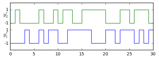
The correlation properties are good as well; if I take a sequence of output bits \( y_1[k] \) from an LFSR and shift it by \( d \) samples to produce a second sequence \( y_2[k] = y_1[k-d] \), then \( y_1 \) and \( y_2 \) have a cross-correlation that is much lower as long as \( d \neq 0 \). Here we define \( y’[k] = 2y[k] - 1 \) so that \( y’[k] \) takes on values of \( \pm1 \) instead of 0 and 1 bits. It’s possible to show that the cross-correlation between \( y’_1[k] \) and \( y’_2[k] \) is two-valued:
$$ \sum\limits _ {k=0}^{2^N-1} y’ _ 1[k]y’ _ 2[k] = \sum\limits _ {k=0}^{2^N-1} y’ _ 1[k]y’ _ 1[k-d] = \begin{cases} 2^N-1 & d = 0 \cr -1 & d \neq 0 \end{cases} $$
from libgf2.gf2 import GF2QuotientRing

H25 = GF2QuotientRing(0x25)

def lfsr_output(field, nsamples=None, init_state=1, shift=0):
    """
    generate nsamples output bits from an LFSR
    (nsamples = None assumes 2^N-1)
    """
    N = field.degree
    if nsamples is None:
        nsamples = (1<<N) - 1
    e = field.rshiftraw(init_state, shift)
    for _ in xrange(nsamples):
        yield e >> (N-1)
        e = field.lshiftraw1(e)

y1 = list(lfsr_output(H25))
print('y1=%s' % y1)
y2 = list(lfsr_output(H25,shift=3))
print('y2=%s' % y2)

# convert from {0,1} to {-1,1}

y1 = np.array(y1)*2-1
y2 = np.array(y2)*2-1
fig = plt.figure(figsize=(6,2))
ax = fig.add_subplot(1,1,1)
ax.plot(y1, drawstyle='steps')
ax.plot(y2+3, drawstyle='steps')
ax.set_ylim(-2,5)
ax.set_yticks([-1,1,2,4])
ax.set_yticklabels([-1,1,-1,1])
ax.text(-1.5,0,'$y_1\'$',fontsize=12)
ax.text(-1.5,3,'$y_2\'$',fontsize=12)
y1=[0, 0, 0, 0, 1, 0, 0, 1, 0, 1, 1, 0, 0, 1, 1, 1, 1, 1, 0, 0, 0, 1, 1, 0, 1, 1, 1, 0, 1, 0, 1]
y2=[1, 0, 1, 0, 0, 0, 0, 1, 0, 0, 1, 0, 1, 1, 0, 0, 1, 1, 1, 1, 1, 0, 0, 0, 1, 1, 0, 1, 1, 1, 0]
We can demonstrate the correlation identity (\( 2^N-1 \) for no shift, \( -1 \) for any other shift) fairly easily:
def circ_correlation(x, y):
    """circular cross-correlation"""
    assert len(x) == len(y)
    return np.correlate(x, np.hstack((y[1:], y)), mode='valid')

H25 = GF2QuotientRing(0x25)
H187 = GF2QuotientRing(0x187)
for H in [H25,H187]:
    y=np.array(list(lfsr_output(H)))*2-1
    print circ_correlation(y,y)
[31 -1 -1 -1 -1 -1 -1 -1 -1 -1 -1 -1 -1 -1 -1 -1 -1 -1 -1 -1 -1 -1 -1 -1 -1 -1 -1 -1 -1 -1 -1] [255 -1 -1 -1 -1 -1 -1 -1 -1 -1 -1 -1 -1 -1 -1 -1 -1 -1 -1 -1 -1 -1 -1 -1 -1 -1 -1 -1 -1 -1 -1 -1 -1 -1 -1 -1 -1 -1 -1 -1 -1 -1 -1 -1 -1 -1 -1 -1 -1 -1 -1 -1 -1 -1 -1 -1 -1 -1 -1 -1 -1 -1 -1 -1 -1 -1 -1 -1 -1 -1 -1 -1 -1 -1 -1 -1 -1 -1 -1 -1 -1 -1 -1 -1 -1 -1 -1 -1 -1 -1 -1 -1 -1 -1 -1 -1 -1 -1 -1 -1 -1 -1 -1 -1 -1 -1 -1 -1 -1 -1 -1 -1 -1 -1 -1 -1 -1 -1 -1 -1 -1 -1 -1 -1 -1 -1 -1 -1 -1 -1 -1 -1 -1 -1 -1 -1 -1 -1 -1 -1 -1 -1 -1 -1 -1 -1 -1 -1 -1 -1 -1 -1 -1 -1 -1 -1 -1 -1 -1 -1 -1 -1 -1 -1 -1 -1 -1 -1 -1 -1 -1 -1 -1 -1 -1 -1 -1 -1 -1 -1 -1 -1 -1 -1 -1 -1 -1 -1 -1 -1 -1 -1 -1 -1 -1 -1 -1 -1 -1 -1 -1 -1 -1 -1 -1 -1 -1 -1 -1 -1 -1 -1 -1 -1 -1 -1 -1 -1 -1 -1 -1 -1 -1 -1 -1 -1 -1 -1 -1 -1 -1 -1 -1 -1 -1 -1 -1 -1 -1 -1 -1 -1 -1 -1 -1 -1 -1 -1 -1 -1 -1 -1 -1 -1 -1]
Why does cross-correlation matter?
Well, one aspect of any PRNG is whether its samples appear to be independent. Of course, in reality they are all dependent because the PRNG is a deterministic state machine, but in an ideal world there should be no dependence in statistical properties of samples \( y[1], y[2], y[3], y[4], \ldots \) given the value of sample \( y[0] \), and one property of independent identically-distributed random variables is that they are uncorrelated, so showing a cross-correlation near zero is a desirable property.
Hmm. I’ve thrown a new term at you twice so far: random variable, which is essentially the ensemble of all possible outcomes of a random sample, kind of like Schrödinger’s cat — this classic quantum physics thought experiment is that you have a cat in a box along with some poison that is triggered randomly through some quantum-mechanical process like radioactive decay. This is an unnaturally well-behaved cat: it stays in the box until further notice, without making a sound or moving around. At any rate, if you look in the box, it is either alive or dead, but until you look inside, the cat is in a superposition of states, and whether the cat is alive or dead is not determined. That’s the idea, anyway.
In our case, a random variable \( b \) might take on values \( 0 \) and \( 1 \) with equal probability, like flipping a fair coin that can produce either heads or tails. This is a Bernoulli distribution, with parameter \( p=\frac{1}{2} \). When you take a sample of the random variable (flipping the coin), then you come up with an actual outcome; before that, it’s just a set of possible outcomes with a probability assigned to each outcome. Suppose we had two independent random variables \( b_1 \) and \( b_2 \), each with the same Bernoulli distribution with \( p=\frac{1}{2} \). The random variables \( b’_1 = 2b_1 - 1 \) and \( b’_2 = 2b_2 - 1 \) are modified distributions with possible outcomes \( -1 \) and \( +1 \) but the same probabilities \( \frac{1}{2} \) in each case. The expected value \( E(b’_1) = E(b’_2) = 0 \): this is just a weighted average over all outcomes, with the weights equal to the probability of each outcome. The correlation of \( b’_1 \) and \( b’_2 \) is defined as \( E((b’_1 - E(b’_1))(b’_2 - E(b’_2)) \) — it’s just the expected value of the product of the deviations of each random variable from its expected value — and is guaranteed to be zero if \( b’_1 \) and \( b’_2 \) are independent. Random variables with zero correlation are called uncorrelated. Since \( b’_1 \) and \( b’_2 \) already have an expected value of zero, then the correlation is just \( E(b’_1b’_2) \). There are four possibilities here, each with probability \( \frac{1}{4} \):
- \( b’_1 = -1, b’_2 = -1 \implies b’_1b’_2 = +1 \)
- \( b’_1 = +1, b’_2 = -1 \implies b’_1b’_2 = -1 \)
- \( b’_1 = -1, b’_2 = +1 \implies b’_1b’_2 = -1 \)
- \( b’_1 = +1, b’_2 = +1 \implies b’_1b’_2 = +1 \)
and the net expected value of their product is zero. But in each of the four cases, the product is either \( +1 \) or \( -1 \).
I’ve just gone through quite a bit of mathematical exposition, but it’s a really important point: the correlation of random variables is a calculation of expected value, and making the same calculations on individual samples will have some variability: the results you get aren’t equal to the expected value, even though the average over a large number of samples is equal. (The fact that the average over a large number of samples converges to the expected value, is a behavior called ergodicity.)
Let’s pretend for a moment that the numpy.random PRNG, which uses the Mersenne Twister algorithm, is perfect in a statistical sense, and use it to generate a bunch of length-255 samples of \( \pm 1 \), and calculate the cross-correlation with each other and with itself (called the autocorrelation function):
# make sure we can reproduce these results
np.random.seed(123)

N=255
y1 = np.random.randint(2,size=N)*2 - 1
Nsamples = 10000
# histograms
hist_cross = {k:0 for k in xrange(-N,N+1,2)}
hist_auto  = {k:0 for k in xrange(-N,N+1,2)}
for _ in xrange(Nsamples):
    y2 = np.random.randint(2,size=N)*2 - 1
    crosscorr = circ_correlation(y1,y2)
    autocorr  = circ_correlation(y2,y2)
    for c in crosscorr:
        hist_cross[c] += 1
    # autocorr[0] is always N since each sample correlates perfectly with itself
    for c in autocorr[1:]:
        hist_auto[c] += 1
def array_of_nonzero_values(hist_dict):
hist = np.array([(k,v) for k,v in hist_dict.iteritems() if v>0])
M = np.abs(hist[:,0]).max()
return hist, M
hist_crossx, Mcross = array_of_nonzero_values(hist_cross)
hist_autox, Mauto = array_of_nonzero_values(hist_auto)
M = max(Mcross, Mauto)
for data, desc in [(hist_crossx, 'Cross-correlation'),
(hist_autox, 'Autocorrelation')]:
fig = plt.figure()
ax = fig.add_subplot(1,1,1)
ax.bar(data[:,0],data[:,1])
ax.set_title('%s values between sample arrays' % desc)
ax.set_xlim(-M,M)
tickspacing = 20
mceil = np.ceil(M/tickspacing)
ax.set_xticks(np.arange(-tickspacing*mceil,tickspacing*mceil+1,tickspacing))
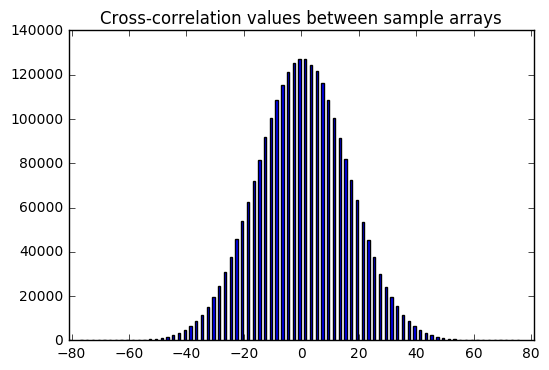
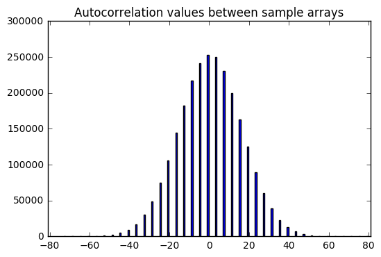
Now that’s interesting. We get these nice bell curve distributions over sample data. It looks like there is a zero expected value of both the cross-correlation and autocorrelation (aside from the correlation with zero shift, which is excluded here) — which makes sense; again, these are supposed to be independent and hence uncorrelated samples, so correlation statistics should have an expected value of zero.
But there is a distribution; sometimes we get cross-correlation or autocorrelation values that are +19 or -33. It depends on luck.
Compare that with the sequence of -1 or +1 outputs derived from LFSR output — it has autocorrelation values (aside from the correlation with zero shift) that are always -1. The LFSR output is really good; it’s very close to zero, much better than perfectly statically random samples.
In fact, it’s too good. By looking at autocorrelation, we can distinguish random-looking LFSR-derived output from a PRNG with good statistical properties, and that means we have an easy statistical test that the LFSR-derived output fails. The output bits of an LFSR are actually more quasi-random than pseudo-random. The classic examples of a quasi-random number generator are the Van der Corput sequence and Halton sequence, which can be used for Monte Carlo analysis due to their “more-even-than-random” space-filling properties:
def halton(base):
    i = 0
    while True:
        i += 1
        f = 1.0
        x = 0
        q = i
        while q > 0:
            f /= base
            q,r = divmod(q,base)
            x += f*r
        yield x

fig = plt.figure(figsize=(8,4))
ax = [fig.add_subplot(1,2,k+1) for k in xrange(2)]
halton2 = halton(2)
halton3 = halton(3)
np.random.seed(123)
for n,m in [(100,'x'),(1000,'o'),(10000,'.')]:
    x = np.array([halton2.next() for _ in xrange(n)])
    y = np.array([halton3.next() for _ in xrange(n)])
    msz = 3.0 if m == 'x' else 2.0
    ax[0].plot(x,y,m,markersize=msz)
    x = np.random.rand(n)
    y = np.random.rand(n)
    ax[1].plot(x,y,m,markersize=msz)
ax[0].set_title('Halton sequences (x=2,y=3)')
ax[1].set_title('np.random.rand')
for axk in ax:
    axk.set_aspect('equal')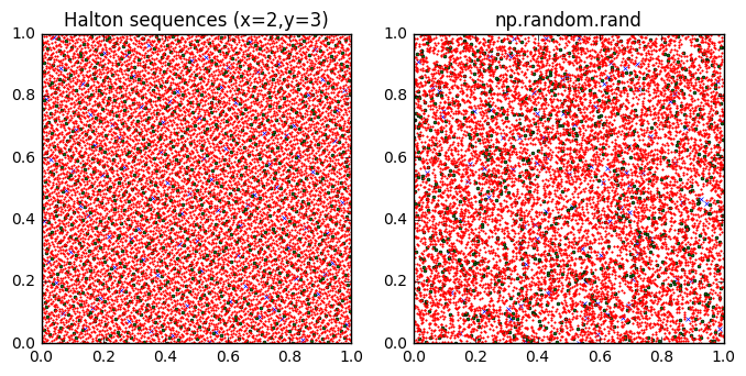
The blue x’s are the first 100 samples; the green circles are the next 1000 samples, and the red dots are the next 10000 samples. The Halton sequences fill the unit square much more evenly than the output of np.random.rand. In fact, I think I see a dog facing to the right sticking its tongue out....
Quasi-random numbers are carefully constructed so that they avoid clustering, whereas with statistically-random numbers you do get clustering. Real randomly-generated numbers exhibit clustering. This is a frequent source of complaints in music-playing programs like iTunes: that some songs repeat several times when others don’t play at all. If you want statistically-random choices, that’s what you get.
In the case of LFSR output bits, the correlation properties aren’t a bug, they’re a feature: yes, the output sequence of an LFSR is distinguishable from statistically-random number generators, but there are reasons to use LFSR output bits specifically for their guarantee of low correlation. We’ll look at some of these reasons in upcoming articles.
For now, though, just be aware that LFSR output bits are different from a good statistically-random PRNG, so if what you want is a statistically-random PRNG, don’t use an LFSR. If you just need a fast hardware PRNG for single bits, and don’t care too much about its statistical properties, the LFSR is fine.
Use of the LFSR state
Now let’s look at using the entire LFSR state as a random-number generator. Here’s an 8-bit LFSR state based on \( H_{187} = x^8 + x^7 + x^2 + x + 1 \):
def lfsr_state(field, nsamples=None, init_state=1, shift=0):
    """
    generate nsamples output bits from an LFSR
    (nsamples = None assumes 2^N-1)
    """
    N = field.degree
    if nsamples is None:
        nsamples = (1<<N) - 1
    e = field.rshiftraw(init_state, shift)
    for _ in xrange(nsamples):
        yield e
        e = field.lshiftraw1(e)

for s in lfsr_state(H187, nsamples=20):
    print s
1 2 4 8 16 32 64 128 135 137 149 173 221 61 122 244 111 222 59 118
Does this look random to you? No! You get a lot of cases where some number \( s \) is immediately followed by \( 2s \). Let’s ignore that problem and look at a few other things.
seq187 = np.array(list(lfsr_state(H187)))
print "mean=%f" % seq187.mean()
print "stdev=%f" % seq187.std()
mean=128.000000
stdev=73.611593
In a statistically-random uniformly distributed random number generator choosing an 8-bit number from 0 to 255, we would expect a mean value of 127.5, and a standard deviation of \( \sqrt{\frac{256^2 + 1}{12}} \approx 73.899 \). Our LFSR output is close to these; the difference is caused by the fact that we never see an all-zero state. If we consider a discrete uniform distribution from 1 to 255, the expected mean and standard deviation would be 128 and \( \sqrt{\frac{255^2 + 1}{12}} \approx 73.607 \), which is almost spot-on. So no problem with those statistics. Let’s plot each number in the sequence against the following number:
seq187_delayed = np.roll(seq187,1)
fig = plt.figure()
ax = fig.add_subplot(1,1,1)
ax.plot(seq187, seq187_delayed, '.')
ax.set_aspect('equal')
ax.set_xlim(0,256)
ax.set_ylim(0,256)
ax.set_xlabel('LFSR output')
ax.set_ylabel('LFSR output, previous value')
<matplotlib.text.Text at 0x11ac825d0>

YUCK! Not random at all. The big line in the lower part of the graph is the equation \( y = x/2 \) and represents all those points where the LFSR state has a high bit of 1 and is therefore followed by a plain left shift. How about an FFT:
np.random.seed(123)
rand255 = np.random.rand(255)*256
def fft_zeromean(x):
    xmean = x.mean()
    return np.abs(np.fft.fft(x-xmean))
plt.plot(fft_zeromean(seq187),'x',label='LFSR output',markersize=3.0)
plt.plot(fft_zeromean(rand255-128.0),'.',label='np.random.rand',markersize=1.0)
plt.xlim(0,255)
plt.legend(labelspacing=0)
<matplotlib.legend.Legend at 0x1235e78d0>
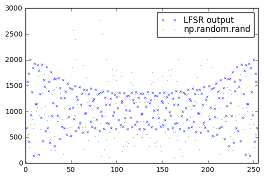
Hmm. That’s not too bad, but the LFSR output does seem to have higher values at lower frequency. Let’s look at a 15-bit LFSR:
H8003 = GF2QuotientRing(0x8003)
seq8003 = np.array(list(lfsr_state(H8003)))
np.random.seed(123)
rand32767 = np.random.rand(32767)*32768
plt.plot(fft_zeromean(seq8003),'x',label='LFSR output',markersize=3.0)
plt.plot(fft_zeromean(rand32767),'.',label='np.random.rand',markersize=1.0)
plt.xlim(0,32767)
plt.legend(labelspacing=0)
<matplotlib.legend.Legend at 0x12120abd0>
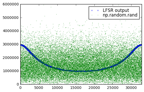
Yeah, that’s not great. We have a definite bias towards lower frequencies; a good PRNG will have relatively even frequency distributions.
Some sources suggest using the lower-order bits of an LFSR; let’s try using the lower 12 bits of this 15-bit LFSR:
H8003 = GF2QuotientRing(0x8003)
seq8003_12 = np.array(list(lfsr_state(H8003))) & 0xFFF
plt.plot(fft_zeromean(seq8003_12),'.',label='LFSR output',markersize=2.0)
plt.xlim(0,32767)
plt.legend(labelspacing=0,loc='best')
<matplotlib.legend.Legend at 0x1331bbdd0>
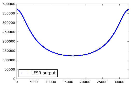
Still not any better. Can we try using fewer bits? Surely some of these must be “random”?
H8003 = GF2QuotientRing(0x8003)
seq8003 = np.array(list(lfsr_state(H8003)))
for k in xrange(1,11):
    m = (1 << k) - 1
    seq8003_k = (seq8003 & m)*1.0/m
    # scale by 1/m so they should all have the same range [0,1]
    plt.plot(fft_zeromean(seq8003_k),label=str(k))
plt.xlim(0,32767)
plt.legend(labelspacing=0, fontsize=10);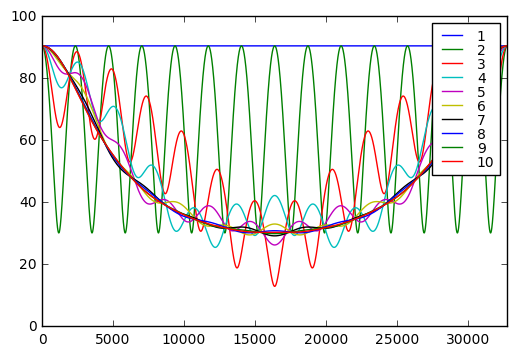
It turns out that if we take bits of the LFSR state, the only number of bits we can use that have a frequency spectrum that is a uniform amplitude as a function of frequency — which is a property that good PRNGs should have — is one. Any more than that, and we get weird behavior in the frequency domain: either a strange oscillation for low bit counts like 2 or 3, or dip at higher frequencies for high bit counts.
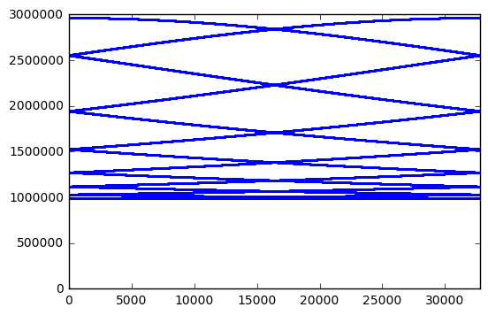
You might think we could fix this. After all, we are taking successive samples of LFSR state, which essentially have an overlap because we shift left by one bit each step. So perhaps we could take every \( N \)th sample, where \( N \) is the bit count, so that there is no overlap between samples of LFSR state. But this is decimation and all it does is to scramble the FFT components, so we have some with higher amplitudes and others with lower amplitudes:
H8003 = GF2QuotientRing(0x8003)
seq8003 = np.array(list(lfsr_state(H8003)))
jj = (np.arange(32767)*15)%32767
seq8003_15 = seq8003[jj]
plt.plot(fft_zeromean(seq8003_15),'.',markersize=3.0)
plt.xlim(0,32767)
print jj[:10]
[ 0 15 30 45 60 75 90 105 120 135]
Perhaps this is just a coincidence, and other bit lengths have better behavior:
for poly in [0x402b, 0x1002d]:
    H = GF2QuotientRing(poly)
    n = H.degree
    m = (1<<n)-1
    assert checkPeriod(H,m) == m
    jj = (np.arange(m)*n)%m
    seq = np.array(list(lfsr_state(H)))
    plt.figure()
    plt.plot(fft_zeromean(seq[jj]),'.',markersize=2.0)
    plt.xlim(0,m)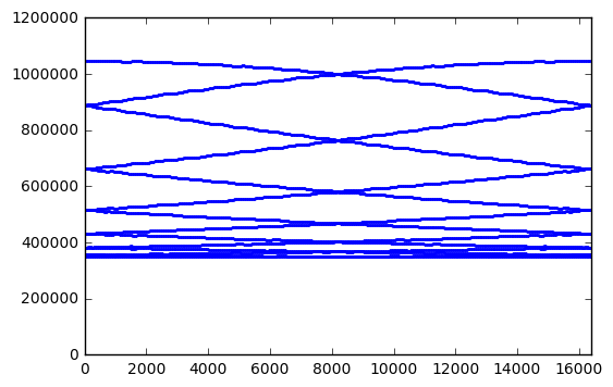
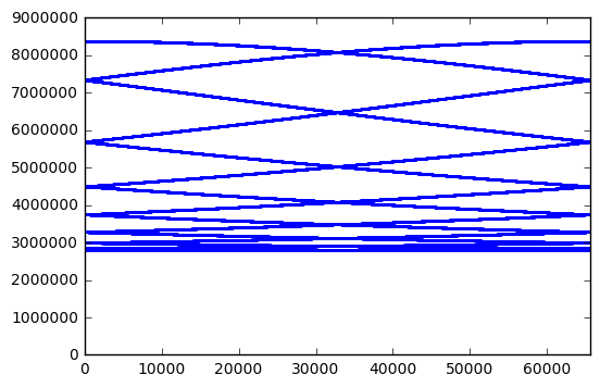
Nope, same issue for 14-bit and 16-bit LFSRs. Anyway, the attraction of using an LFSR goes away if we have to update the state 14 times just to get one random sample. There are many other PRNGs that are simple and fast which have better statistical behavior, like PCG or xorshift.
Does this mean you can’t use LFSR state as a PRNG? No, you just have to understand and accept that it is a substandard PRNG, and it has certain limitations, like high correlation between successive samples, and odd behavior in the frequency domain. Again, look at the other well-established PRNGs and see if they’re suitable.
One more pretty picture for today: we saw in one of the figures that the FFT of the least significant bit of LFSR state has unit amplitude. The same is true for LFSR output (which is the most significant bit of LFSR state). If we look at the FFT output directly as a complex number, and plot it in the complex plane rather than a function of frequency, we get irregular samples of a circle:
seq = np.array(list(lfsr_output(GF2QuotientRing(0x187))))
seqm = seq - seq.mean()
fseq = np.fft.fft(seqm)
plt.plot(np.real(fseq),np.imag(fseq),'.')
plt.axis('equal')
(-8.0, 10.0, -8.0, 8.0)
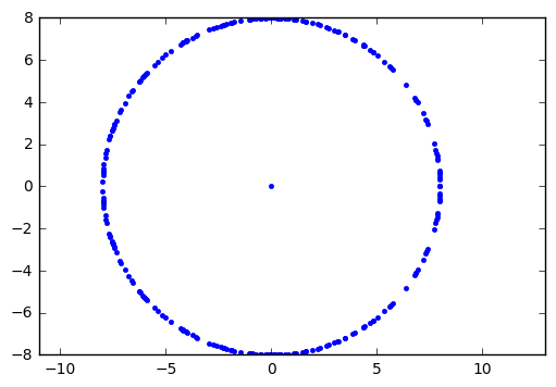
The dot in the center is the DC component, since we subtracted out the mean value before taking the FFT.
Wrapup
We covered the use of LFSRs in random number generation. Actually, LFSRs have limited use in random bit generation, with some statistical oddities that are tolerable and even desirable in certain applications. Specifically, we looked at the autocorrelation function of an LFSR, which is two-valued, showing perfect correlation with no shift (true for any sequence) and almost zero correlation with all other shift values.
As random number generators, using multiple state bits, they show very poor serial correlation properties. Attempts to fix this by using a subset of bits, or batches of bits, still show anomalies in the frequency domain.
Next time we’ll look at spread-spectrum applications. This is an area where LFSRs really shine, and I hope you’ve had the patience to follow this series so far.
References
The standard general references for random number generation are
-
Donald Knuth, The Art of Computer Programming, Volume 2 (Seminumerical Algorithms) — there is a whole chapter of almost 200 pages on random number generation. LFSRs are mentioned in passing (although not by name), for a page or so, but if you want a good background on random number generation, read this. Read it again every few years and maybe by the time you retire you will understand it all.
-
William H. Press, Brian P. Flannery, Saul A. Teukolsky, William T. Vetterling, Numerical Recipes in C — chapter 7 is on random number generation, with one section called “Generation of Random Bits” that is based on LFSRs, although it doesn’t contain any concepts that aren’t presented in this series. The rest of chapter 7 is worth a read.
Other references:
- George Marsaglia, Random Numbers Fall Mainly in the Planes. Proceedings of the National Academy of Sciences, vol. 61, no. 1, pp. 25-28, 1968.
© 2017 Jason M. Sachs, all rights reserved.
- Comments
- Write a Comment Select to add a comment
To post reply to a comment, click on the 'reply' button attached to each comment. To post a new comment (not a reply to a comment) check out the 'Write a Comment' tab at the top of the comments.
Please login (on the right) if you already have an account on this platform.
Otherwise, please use this form to register (free) an join one of the largest online community for Electrical/Embedded/DSP/FPGA/ML engineers:


